Imaging Data and Transforms
Oscar Esteban <phd@oscaresteban.es>
Research & Teaching Ambizione Fellow
Lausanne University Hospital and University of Lausanne
import numpy as np
import nibabel as nb

ni_img = nb.load(
    "/data/datasets/hcph/sub-001/ses-001/anat/"
    "sub-001_ses-001_acq-undistorted_T1w.nii.gz"
)
data = np.asanyarray(
    nb.as_closest_canonical(
        ni_img
    ).dataobj
)
|
Learning outcomes
- Gain an introductory understanding of different types of neuroimaging data.
- Explore the use of Python libraries like NiBabel for working with neuroimaging data formats.
- Understand the importance of image alignment and learn about spatial transforms in this context.
- Discover how to apply these tools and concepts to enhance your own data analysis and interpretation.
Types of Neuroimaging Data
Imaging the Brain's Blueprint: Structural MRI
Maps anatomical features of the brain.
For example, brain tissues:
- Grey matter (information processing)
- White matter (communications)
- Cerebrospinal fluid (support)

Decoding Brain Activity: Functional MRI (fMRI)
Functional MRI measures brain activity indirectly by tracking changes in blood flow, which is linked to neuronal activity:
- Brain regions activated during specific tasks?
- Regions that activate with similar patterns
Mapping white matter: diffusion MRI (dMRI)
Investigates the structure and connectivity of white matter by measuring the diffusion of water molecules.
- The orientation and organization of white matter fiber tracts.
- Tissue microstructure
Digital 3D images
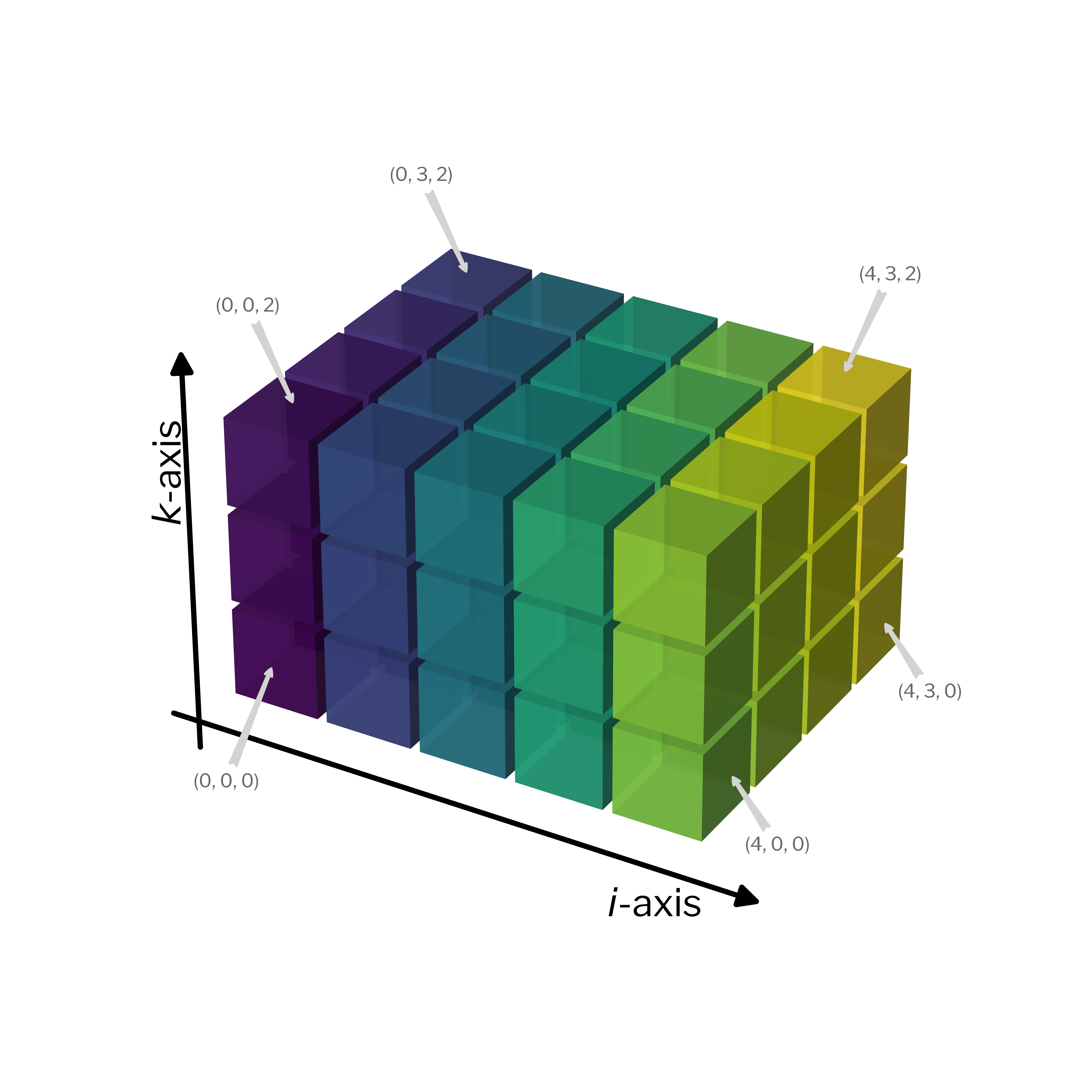
A 3D image
shape = (5, 4, 3)
size = np.prod(shape)
n_voxels = np.arange(1, size + 1).reshape(shape)
>>> shape = (5, 4, 3)
>>> size = np.prod(shape)
>>> size
60
>>> n_voxels = np.arange(
...     1,
...     size + 1,
... ).reshape(shape)
>>> n_voxels[-1, -1, -1]
60
|
 |
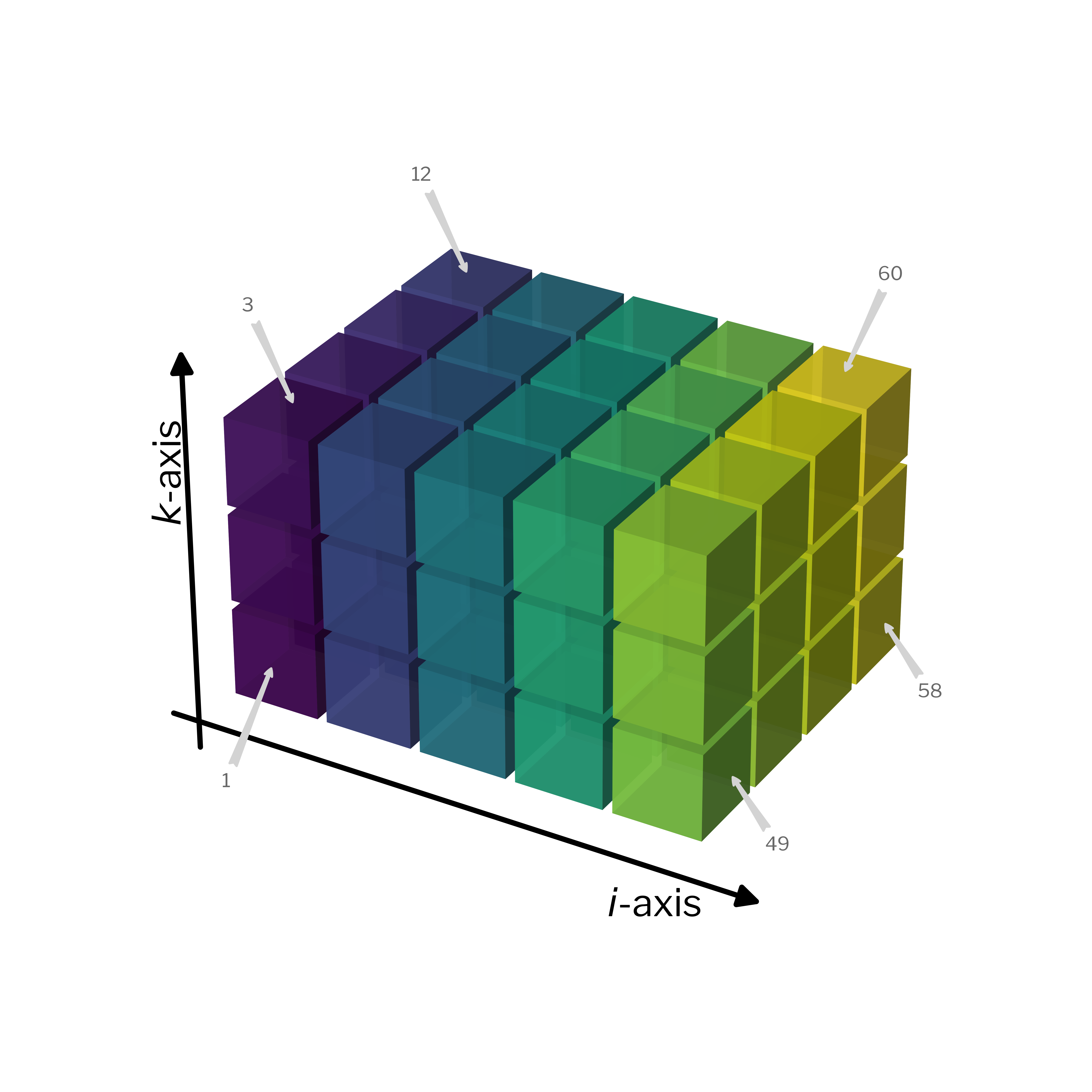
>>> shape = (5, 4, 3)
>>> size = np.prod(shape)
>>> size
60
>>> n_voxels = np.arange(
...     1,
...     size + 1,
... ).reshape(shape)
>>> n_voxels[-1, -1, -1]
60
|
 |
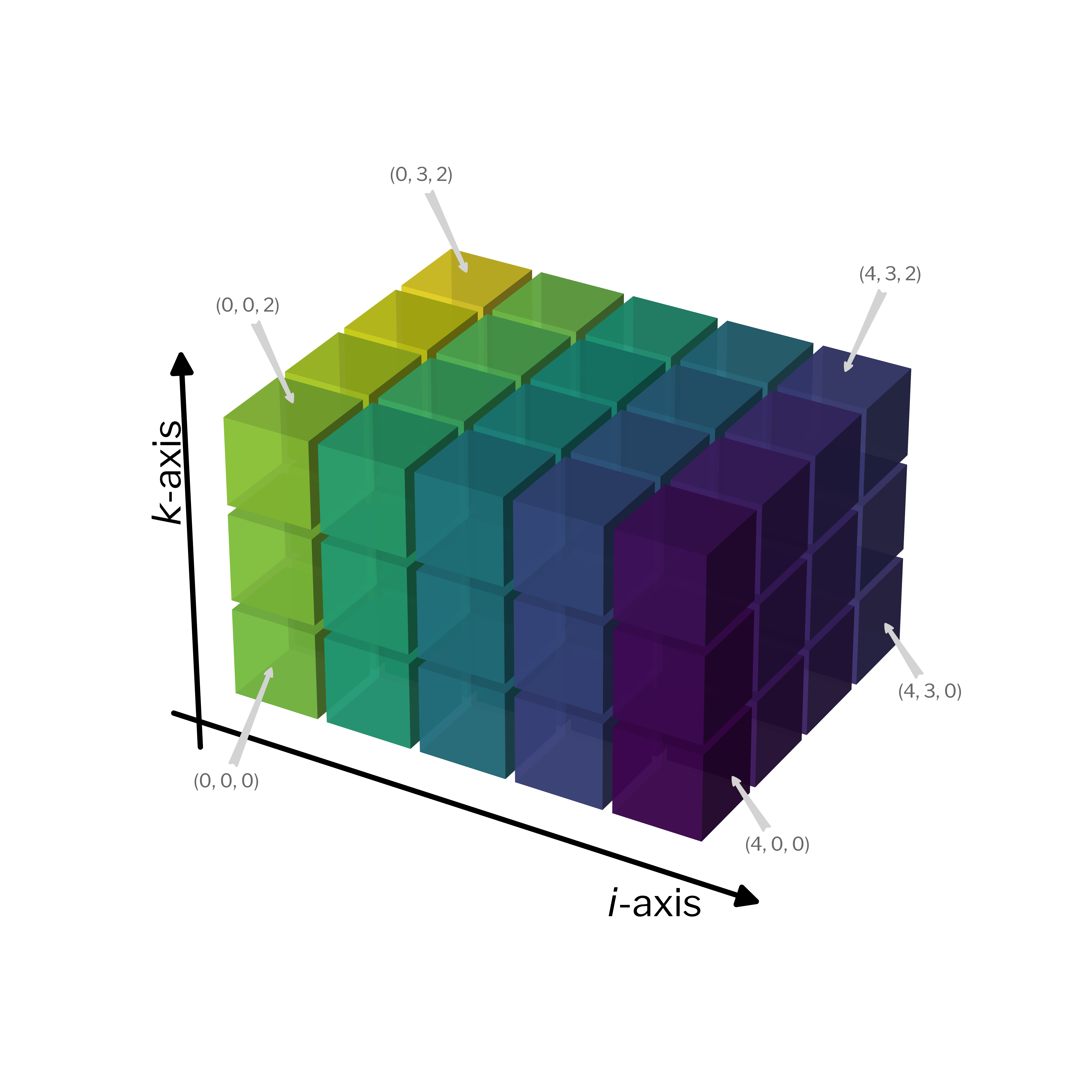
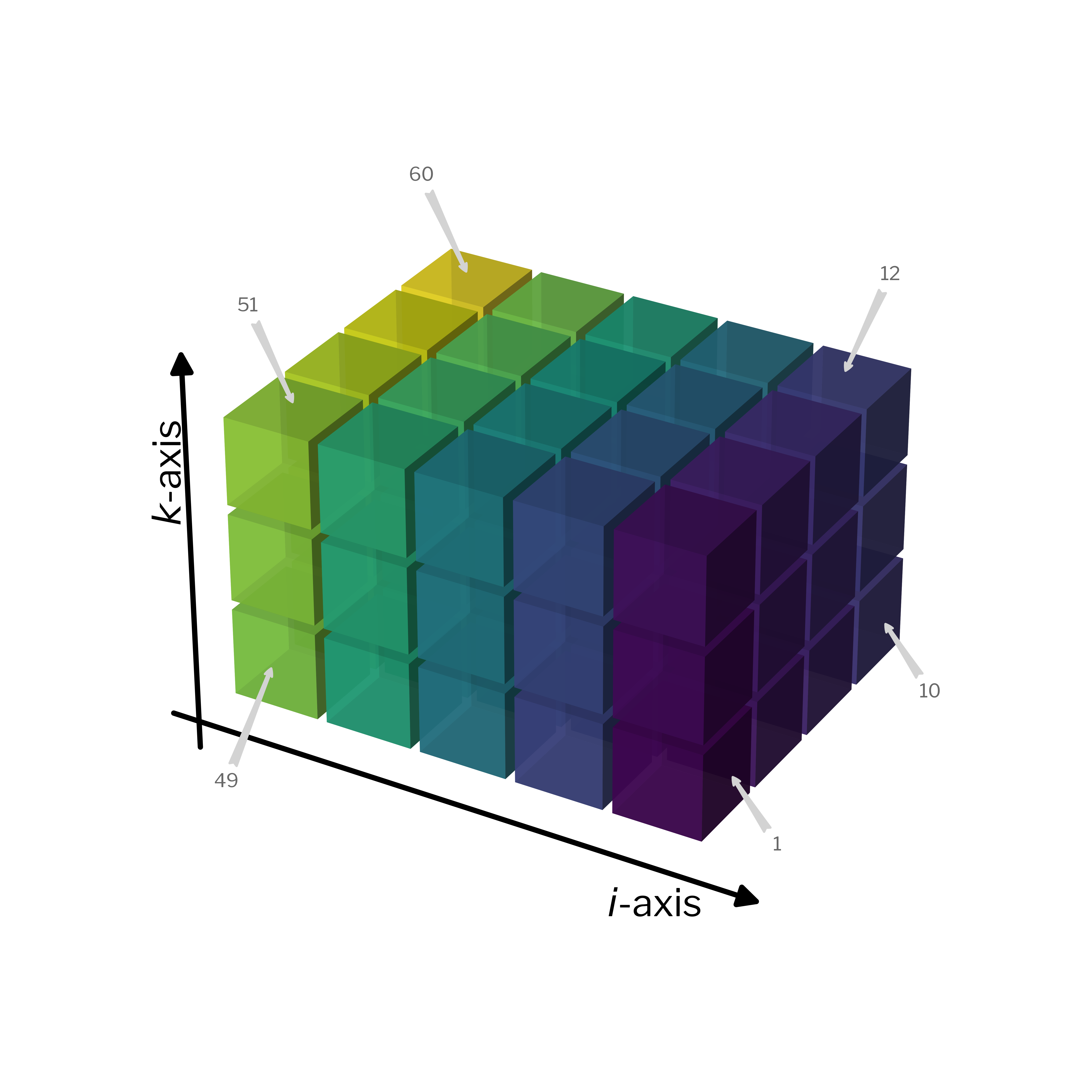
>>> n_voxels[:, 0, 0]
[ 1 13 25 37 49]
|
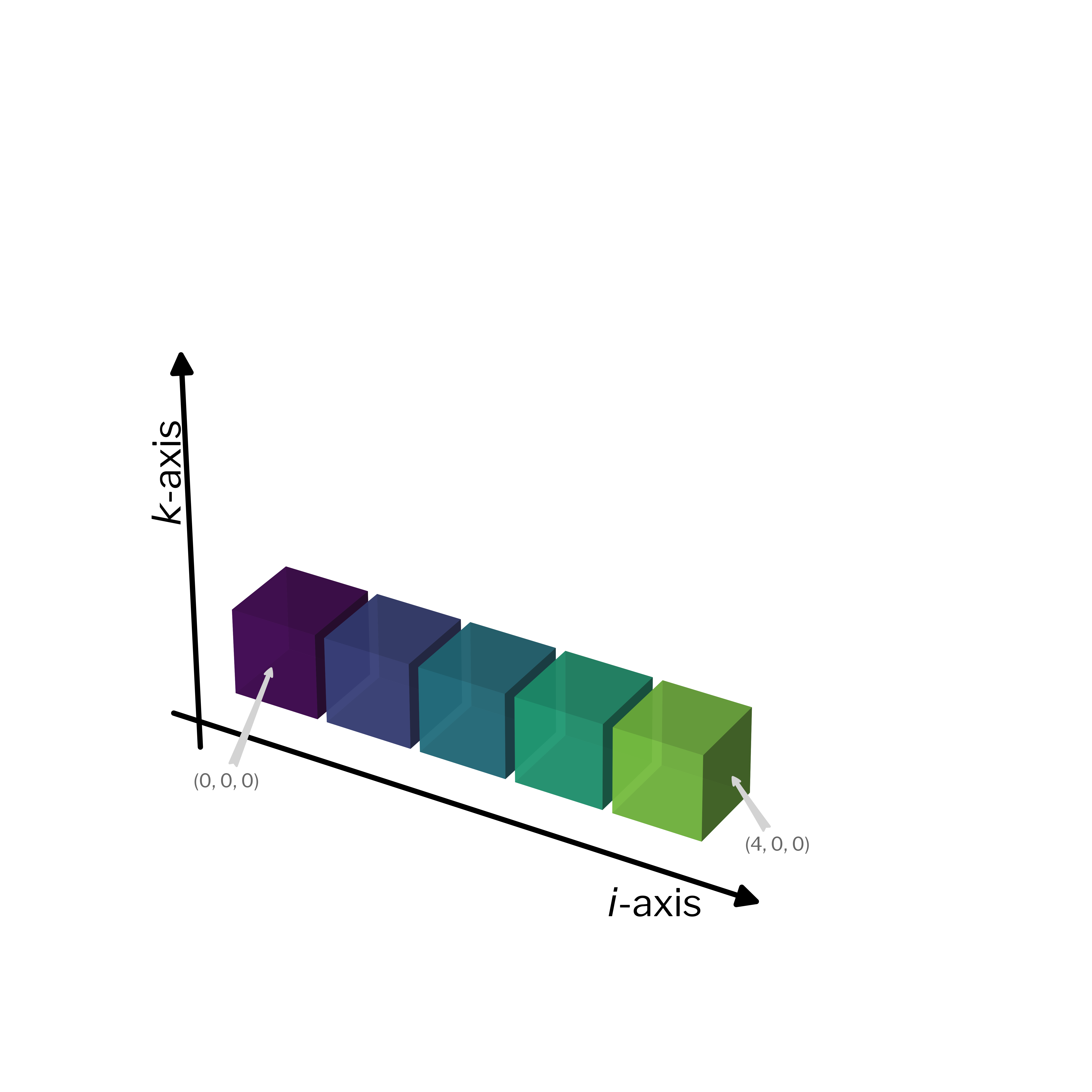 |
>>> n_voxels[:, 0, 0]
[ 1 13 25 37 49]
|
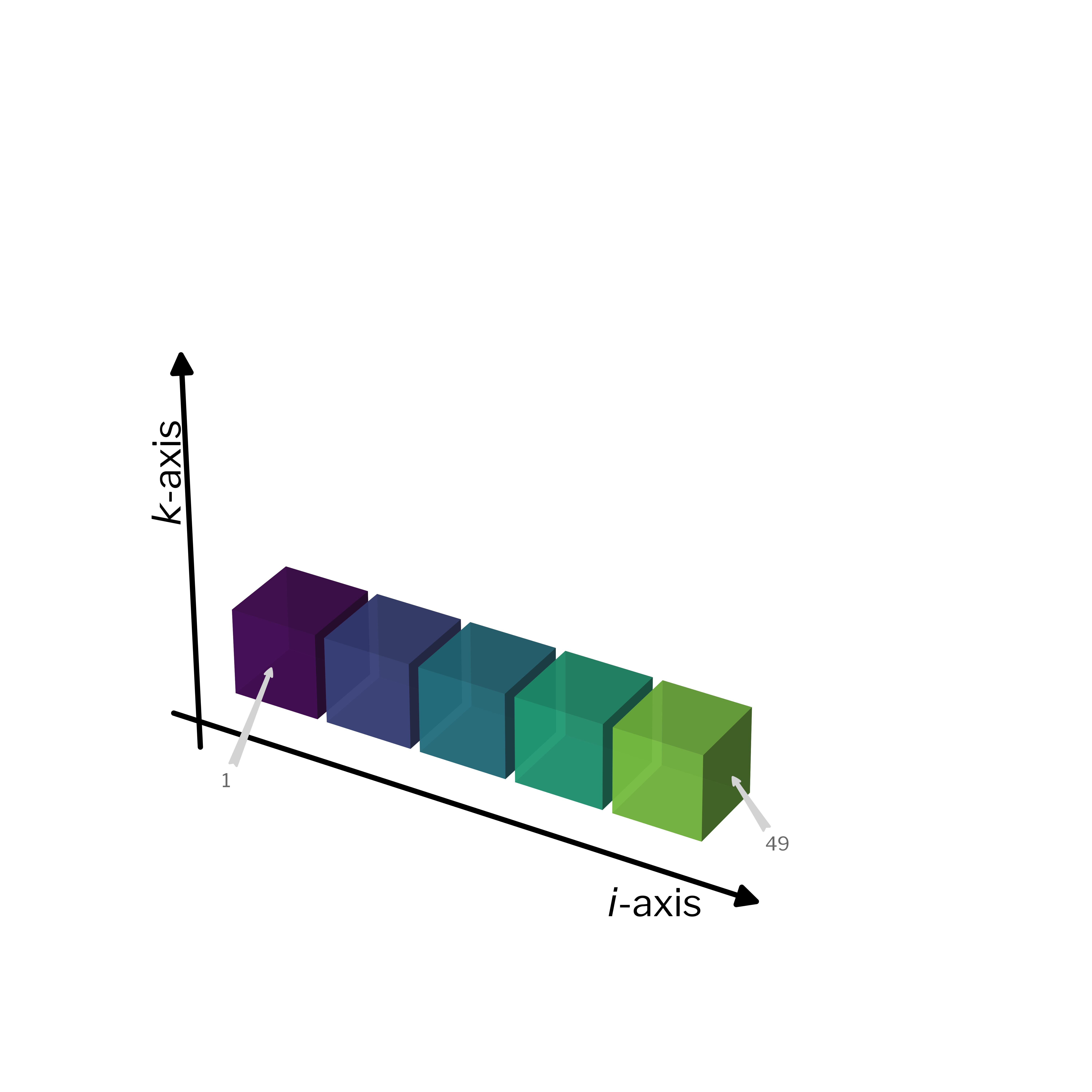 |
>>> n_voxels[:, :1, 0]
[[ 1  4]
 [13 16]
 [25 28]
 [37 40]
 [49 52]]
|
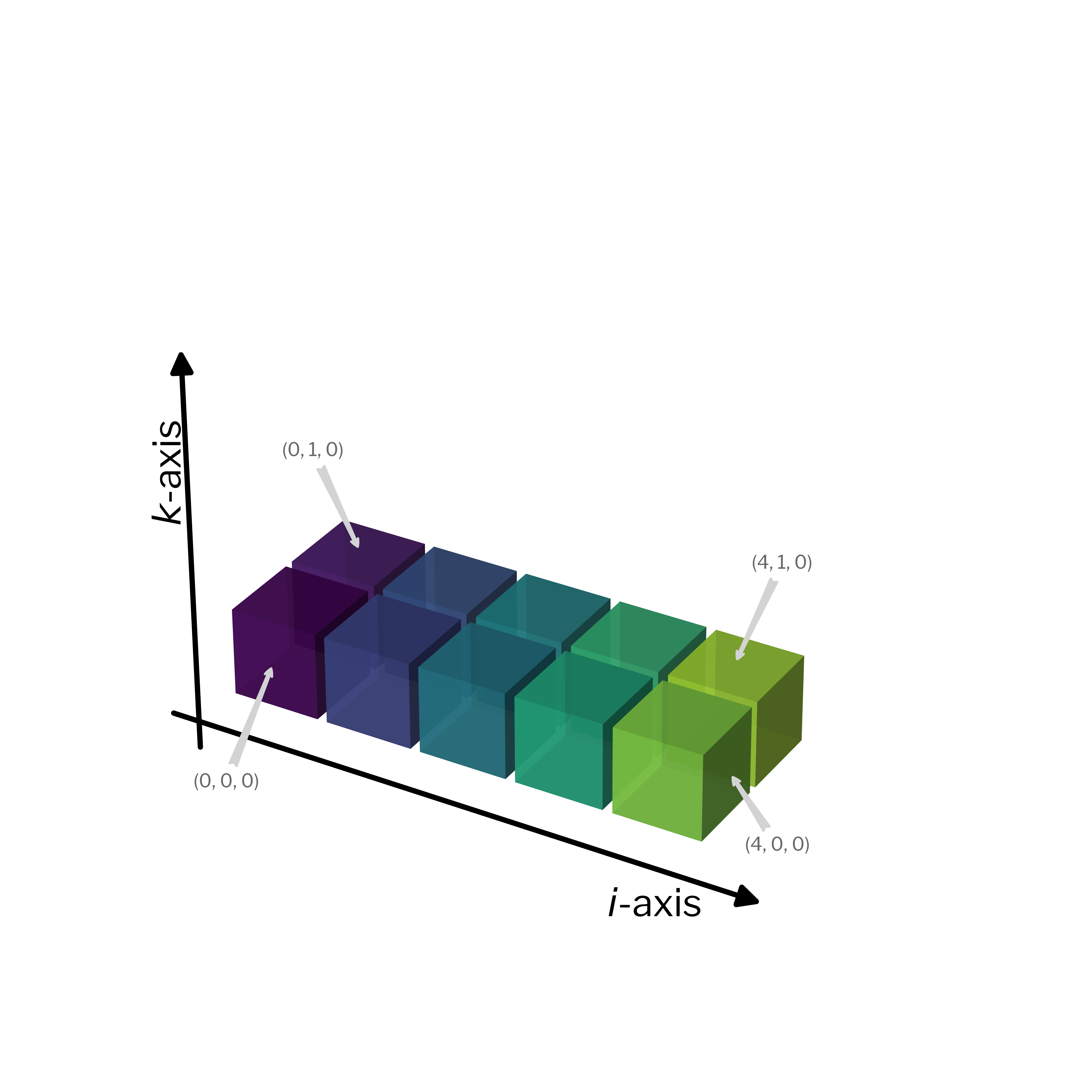 |
>>> n_voxels[:, :1, 0]
[[ 1  4]
 [13 16]
 [25 28]
 [37 40]
 [49 52]]
|
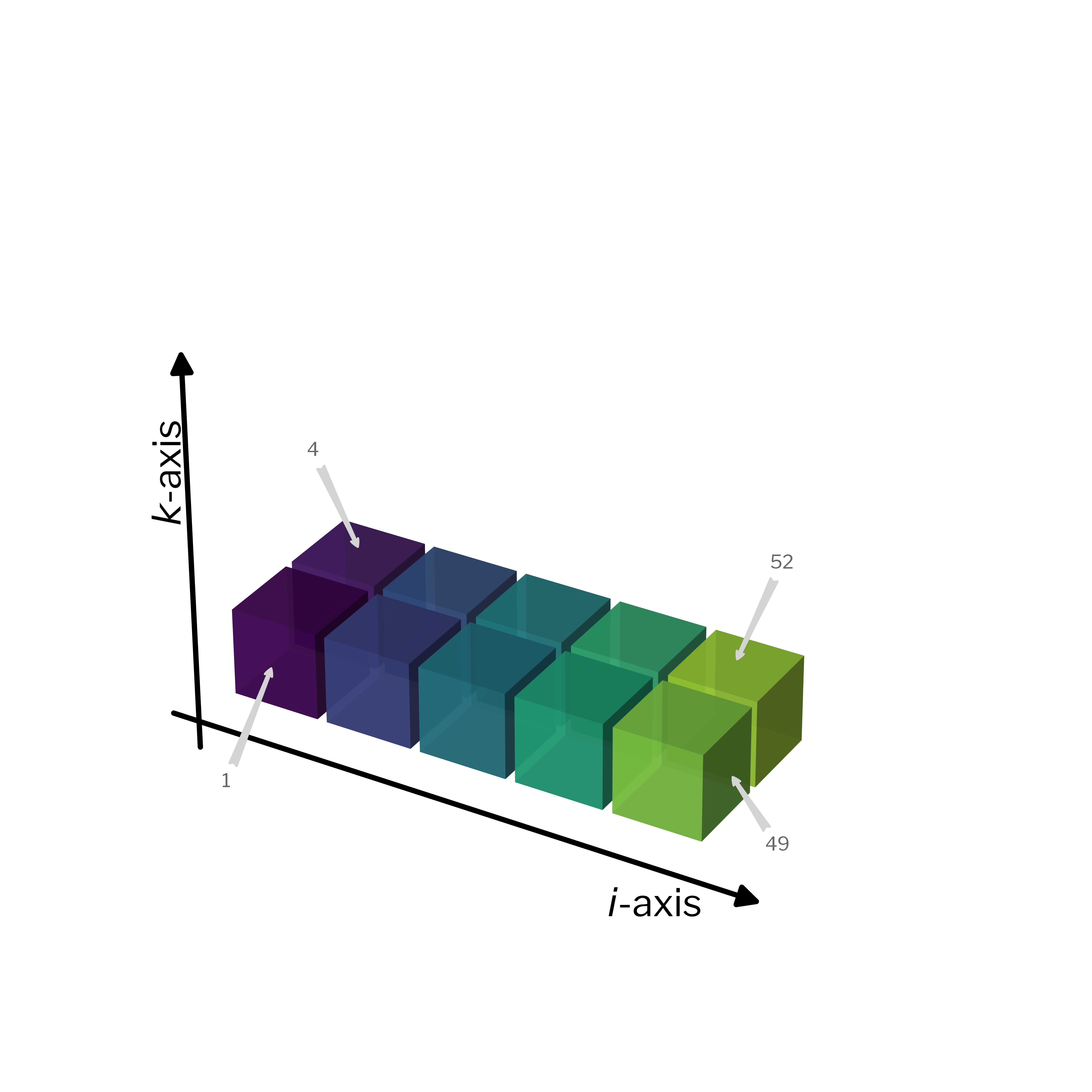 |
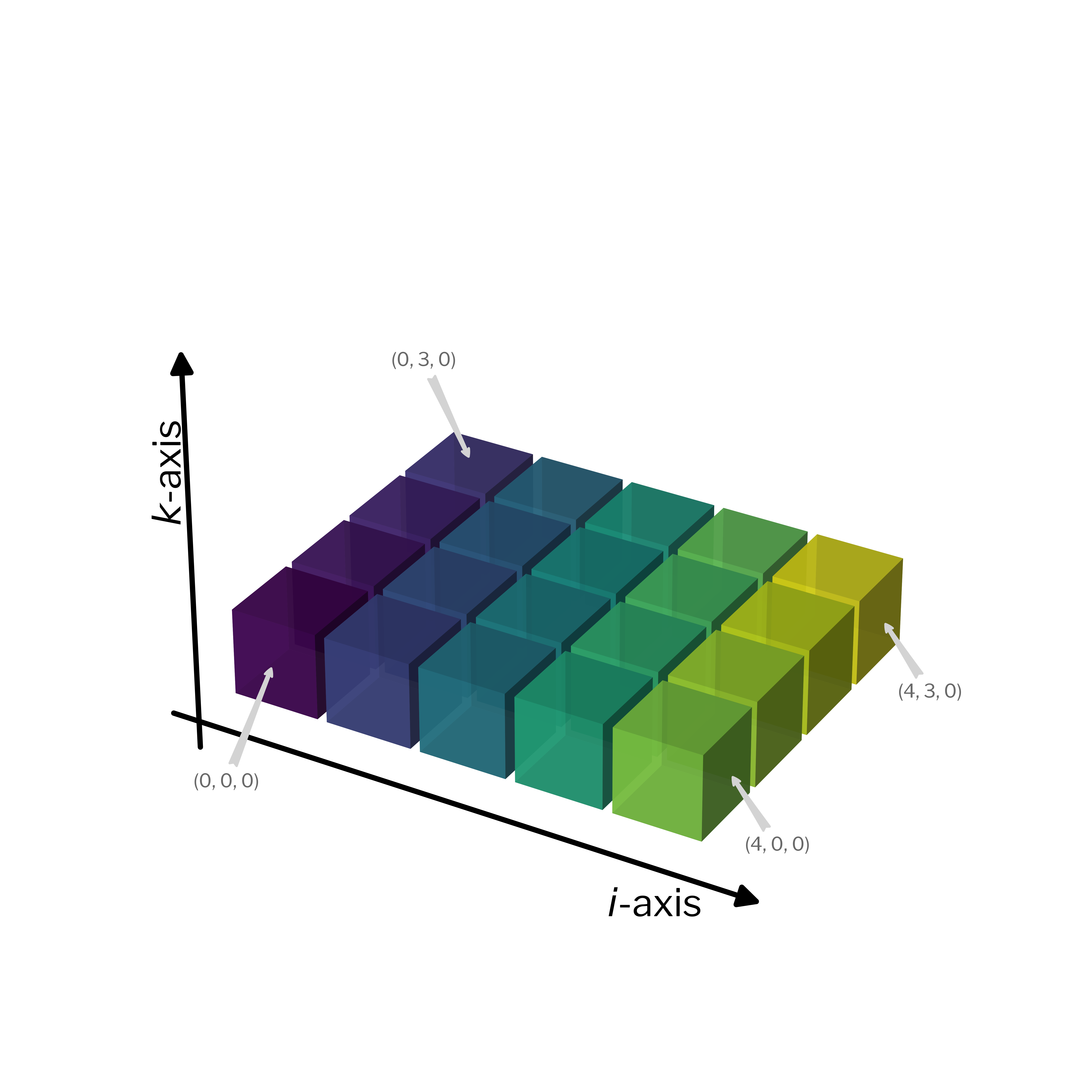
>>> n_voxels[..., 0]
[[ 1  4  7 10]
 [13 16 19 22]
 [25 28 31 34]
 [37 40 43 46]
 [49 52 55 58]]
|
 |
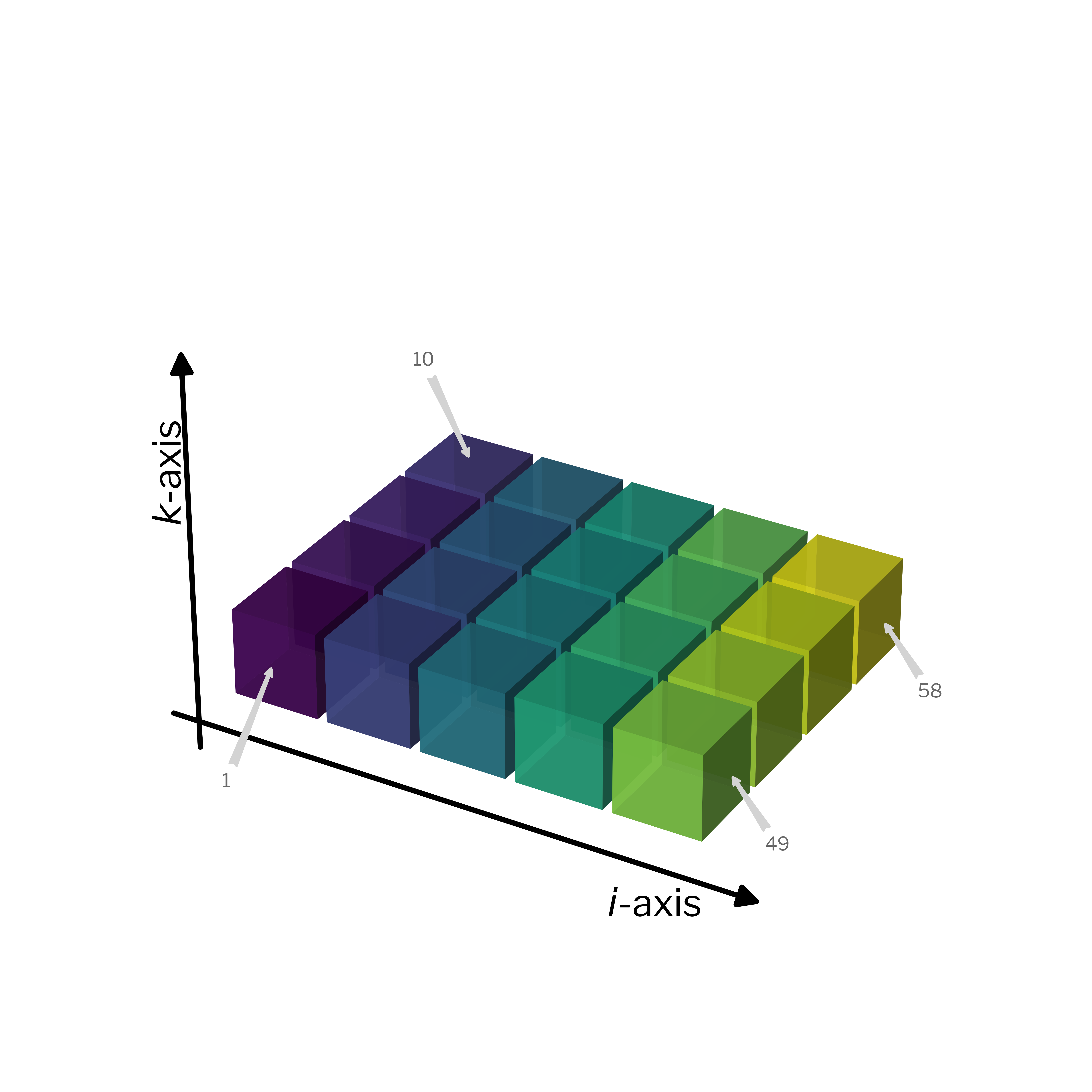
>>> n_voxels[..., 0]
[[ 1  4  7 10]
 [13 16 19 22]
 [25 28 31 34]
 [37 40 43 46]
 [49 52 55 58]]
|
 |
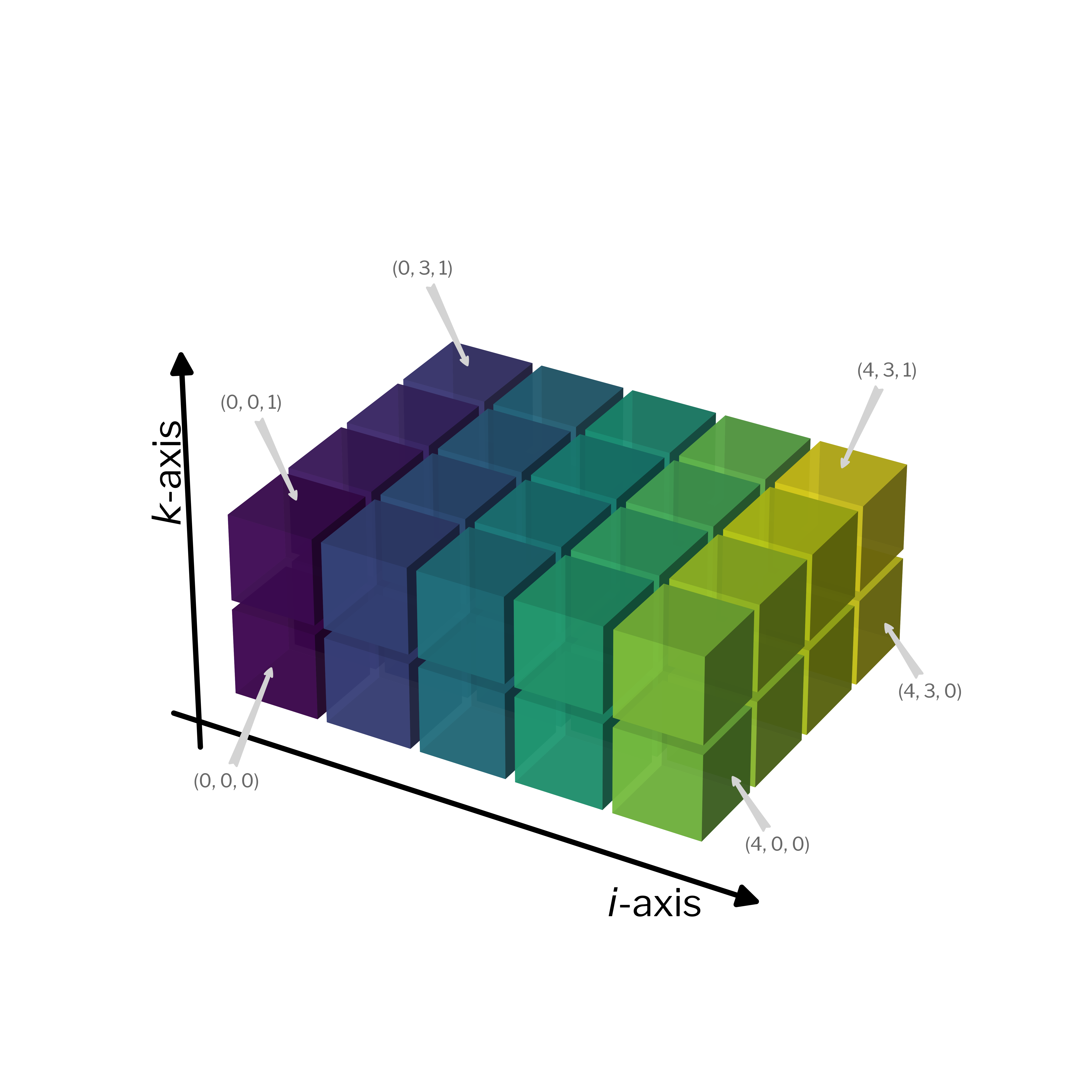
>>> n_voxels[..., :2]
[[[ 1  2]
  [ 4  5]
  [ 7  8]
  [10 11]]

 [[13 14]
  [16 17]
  [19 20]
  [22 23]]

 [[25 26]
  [28 29]
  [31 32]
  [34 35]]

 [[37 38]
  [40 41]
  [43 44]
  [46 47]]

 [[49 50]
  [52 53]
  [55 56]
  [58 59]]]
|
 |
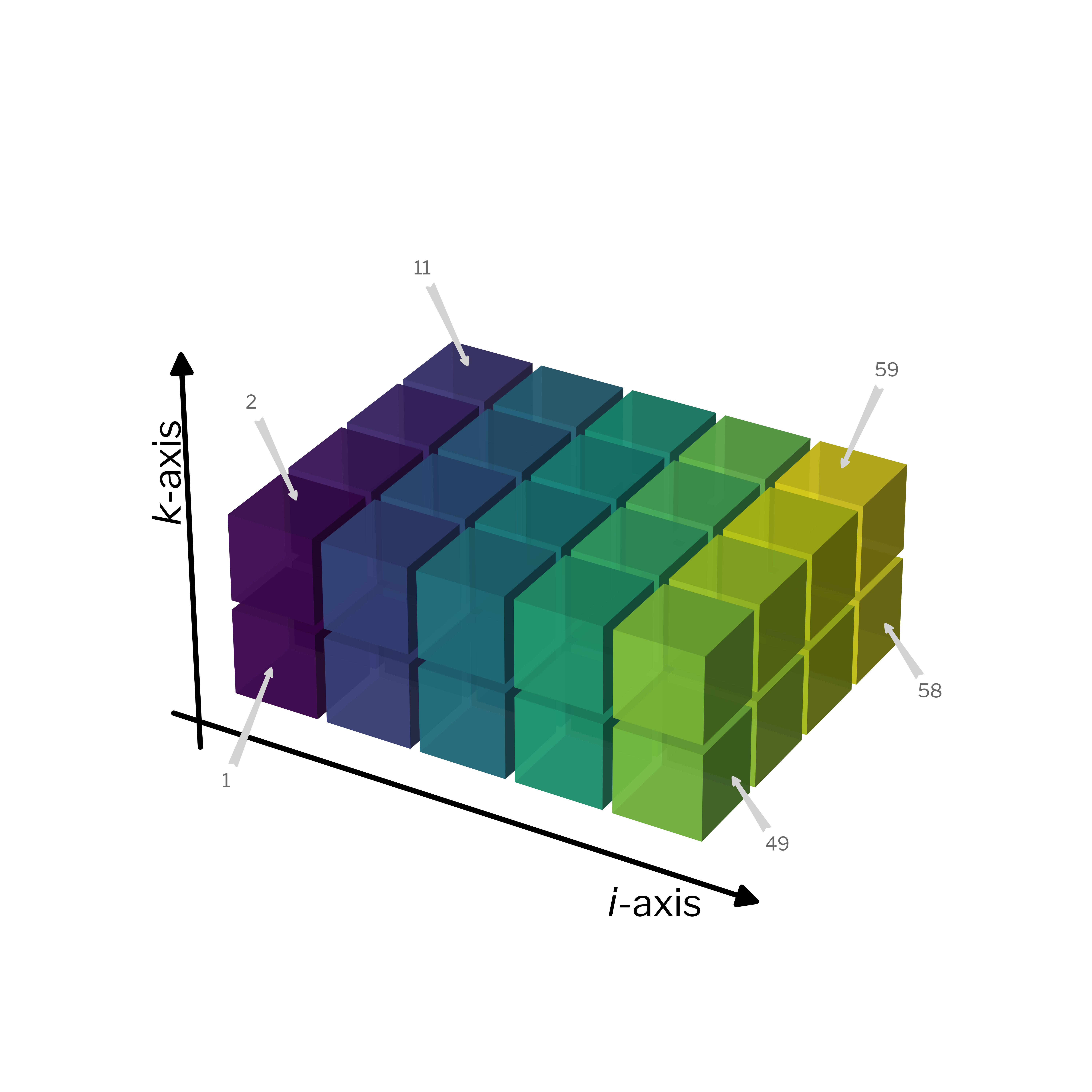
>>> n_voxels[..., :2]
[[[ 1  2]
  [ 4  5]
  [ 7  8]
  [10 11]]

 [[13 14]
  [16 17]
  [19 20]
  [22 23]]

 [[25 26]
  [28 29]
  [31 32]
  [34 35]]

 [[37 38]
  [40 41]
  [43 44]
  [46 47]]

 [[49 50]
  [52 53]
  [55 56]
  [58 59]]]
|
 |
>>> n_voxels = np.flip(
...     n_voxels,
...     axis=0,
... )
>>> n_voxels[:, 0, 0]
[49 37 25 13  1]
|
 |
>>> n_voxels = np.flip(
...     n_voxels,
...     axis=0,
... )
>>> n_voxels[:, 0, 0]
[49 37 25 13  1]
|
 |
>>> n_voxels = np.flip(
...     n_voxels,
...     axis=0,
... )
>>> n_voxels[:, 0, -1]
[51 39 27 15  3]
|
|
>>> n_voxels[1, ...]
[[13 14 15]
 [16 17 18]
 [19 20 21]
 [22 23 24]]
|
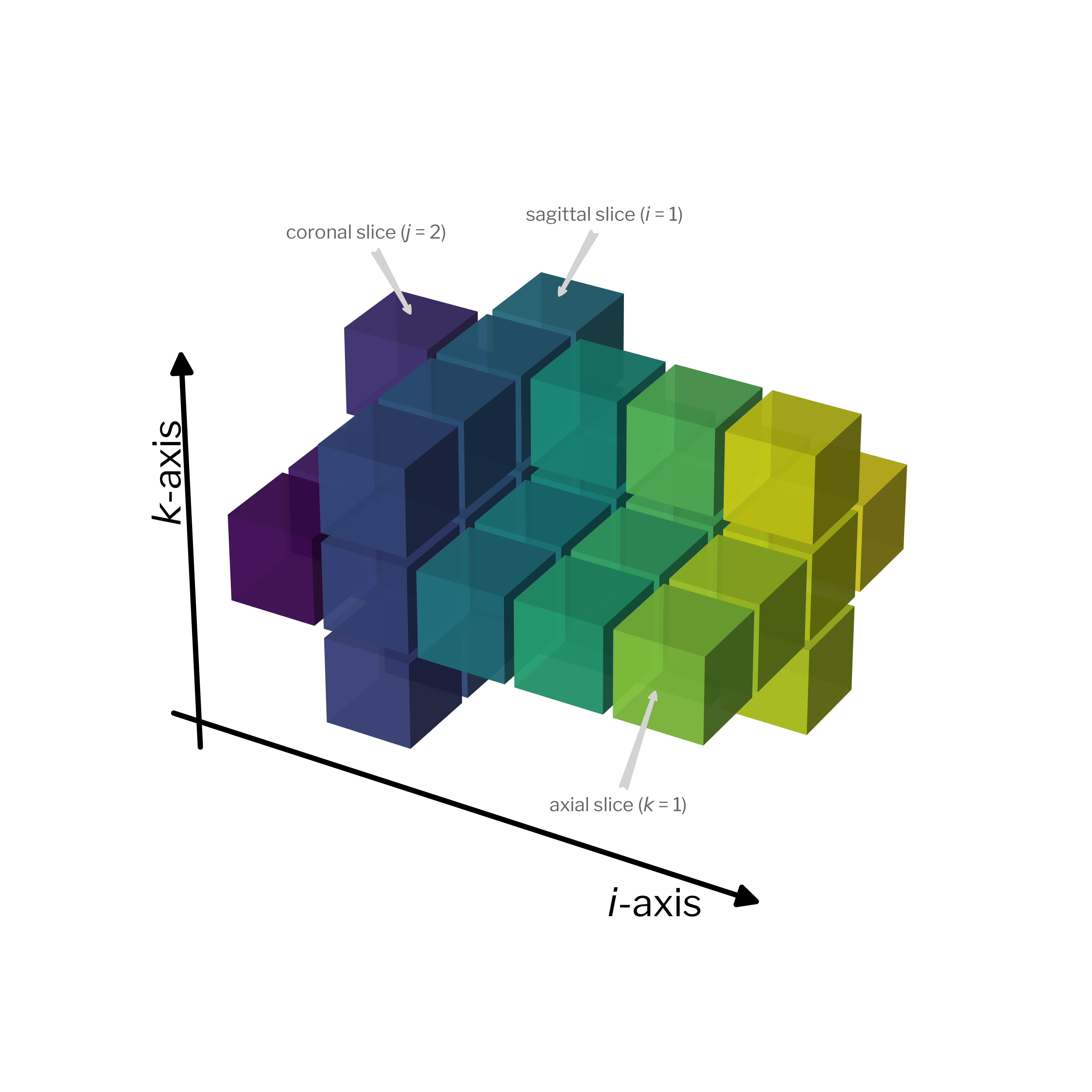 |
>>> n_voxels[:, 2, :]
[[ 7  8  9]
 [19 20 21]
 [31 32 33]
 [43 44 45]
 [55 56 57]]
|
|
>>> n_voxels[..., 1]
[[ 2  5  8 11]
 [14 17 20 23]
 [26 29 32 35]
 [38 41 44 47]
 [50 53 56 59]]
|
|
>>> n_voxels.ravel()
[ 1  2  3  4  5  6  7  8  9 10 11 12 13 14 15 16 17 18 19 20 21 22 23 24
 25 26 27 28 29 30 31 32 33 34 35 36 37 38 39 40 41 42 43 44 45 46 47 48
 49 50 51 52 53 54 55 56 57 58 59 60]
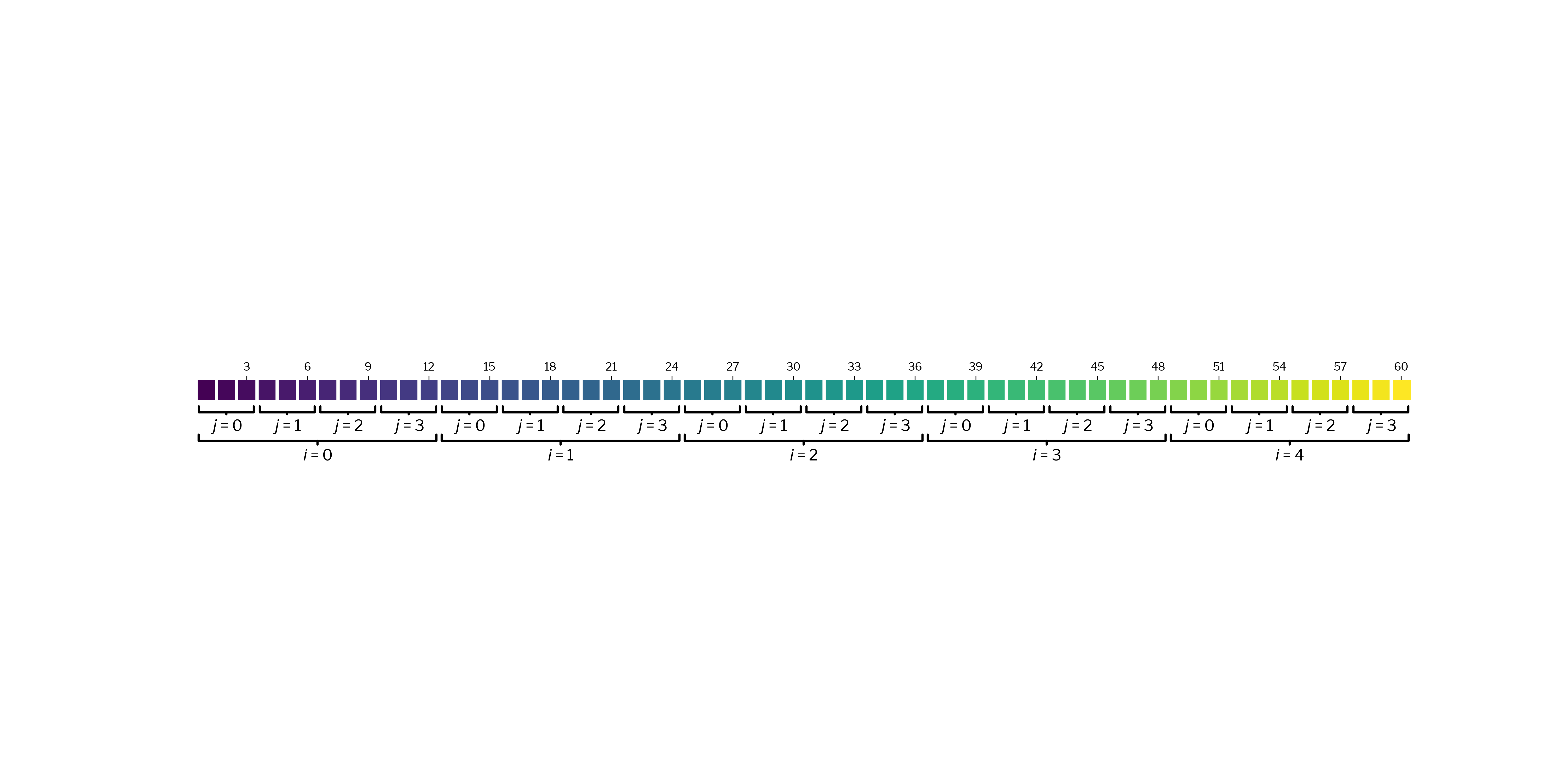
>>> n_voxels.reshape(-1)
[ 1  2  3  4  5  6  7  8  9 10 11 12 13 14 15 16 17 18 19 20 21 22 23 24
 25 26 27 28 29 30 31 32 33 34 35 36 37 38 39 40 41 42 43 44 45 46 47 48
 49 50 51 52 53 54 55 56 57 58 59 60]
>>> n_voxels.reshape(-1)[2::3]
[ 3  6  9 12 15 18 21 24 27 30 33 36 39 42 45 48 51 54 57 60]

NIfTI: Neuroimaging Informatics Technology Initiative
|
import numpy as np
import nibabel as nb

ni_img = nb.load(
    "/data/datasets/hcph/sub-001/ses-001/anat/"
    "sub-001_ses-001_acq-undistorted_T1w.nii.gz"
)
header = ni_img.header
data = np.asanyarray(
    nb.as_closest_canonical(ni_img).dataobj
)
|
>>> ni_img.header
<class 'nibabel.nifti1.Nifti1Header'> object, endian='<'
sizeof_hdr      : 348
data_type       : b''
db_name         : b''
extents         : 0
session_error   : 0
regular         : b'r'
dim_info        : 54
dim             : [  3 252 288 192   1   1   1   1]
intent_p1       : 0.0
intent_p2       : 0.0
intent_p3       : 0.0
intent_code     : none
datatype        : int16
bitpix          : 16
slice_start     : 0
pixdim          : [1.       0.798611 0.798611 0.8      2.2      0.       0.       0.      ]
vox_offset      : 0.0
scl_slope       : nan
scl_inter       : nan
slice_end       : 0
slice_code      : unknown
xyzt_units      : 10
cal_max         : 0.0
cal_min         : 0.0
slice_duration  : 0.0
toffset         : 0.0
glmax           : 0
glmin           : 0
descrip         : b'TE=2.5;Time=183714.883'
aux_file        : b''
qform_code      : scanner
sform_code      : scanner
quatern_b       : -2e-06
quatern_c       : 2e-06
quatern_d       : -1.5514998e-12
qoffset_x       : -100.12736
qoffset_y       : -88.09236
qoffset_z       : -65.619385
srow_x          : [ 7.9861099e-01 -3.9107979e-12  3.2000121e-06 -1.0012736e+02]
srow_y          : [-8.8669775e-12  7.9861099e-01  3.2000121e-06 -8.8092361e+01]
srow_z          : [-3.1944439e-06 -3.1944439e-06  8.0000305e-01 -6.5619385e+01]
intent_name     : b''
magic           : b'n+1'
Querying some metadata
The NIfTI header contains relevant metadata to interpret the image:
>>> ni_img.header.get_xyzt_units()
('mm', 'sec')
>>> ni_img.header.get_data_dtype()
int16
but perhaps the most important metadata is the orientation.
NIfTI stores orientation within two fields:
ni_img.header.get_qform()
[[ 7.98610985e-01 -3.91079826e-12  3.20000004e-06 -1.00127357e+02]
 [-8.86697744e-12  7.98610985e-01  3.20000004e-06 -8.80923615e+01]
 [-3.19444393e-06 -3.19444393e-06  8.00000012e-01 -6.56193848e+01]
 [ 0.00000000e+00  0.00000000e+00  0.00000000e+00  1.00000000e+00]]
ni_img.header.get_sform()
[[ 7.98610985e-01 -3.91079790e-12  3.20001209e-06 -1.00127357e+02]
 [-8.86697746e-12  7.98610985e-01  3.20001209e-06 -8.80923615e+01]
 [-3.19444393e-06 -3.19444393e-06  8.00003052e-01 -6.56193848e+01]
 [ 0.00000000e+00  0.00000000e+00  0.00000000e+00  1.00000000e+00]]
NiBabel gives the best affine with a specific property:
>>> ni_img.affine
[[ 7.98610985e-01 -3.91079790e-12  3.20001209e-06 -1.00127357e+02]
 [-8.86697746e-12  7.98610985e-01  3.20001209e-06 -8.80923615e+01]
 [-3.19444393e-06 -3.19444393e-06  8.00003052e-01 -6.56193848e+01]
 [ 0.00000000e+00  0.00000000e+00  0.00000000e+00  1.00000000e+00]]
Affine transforms
$T\colon R \subset \mathbb{R}^n \to M \subset \mathbb{R}^n$
$\vec{x} \mapsto \vec{x}' = f(\vec{x}).$
where
$\vec{x}' = \begin{pmatrix} 0.798 & 0.000 & 0.001 \\ 0.000 & 0.798 & 0.001 \\ -0.001 & -0.001 & 8.001 \end{pmatrix} \cdot \vec{x} + \begin{pmatrix} -100.130 \\ -88.100 \\ -65.620 \end{pmatrix}$
Using homogeneous coordinates, we can express the affine transform more compactly:
$\begin{pmatrix}x'_0 \\ x'_1 \\ x'_2 \\ 1.0 \end{pmatrix} = \begin{pmatrix} 0.798 & 0.000 & 0.001 & -100.130 \\ 0.000 & 0.798 & 0.001 & -88.100 \\ -0.001 & -0.001 & 8.001 & -65.620 \\ 0 & 0 & 0 & 1 \end{pmatrix} \cdot \begin{pmatrix}x_0 \\ x_1 \\ x_2 \\ 1.0 \end{pmatrix}$
Let's plot our initial image with a more flexible tool
The NIfTI affine
Converts, as any transform, from one coordinate system (voxels) into another (physical coordinates).
Let's define our own NIfTI affine:
$\begin{pmatrix}x \\ y \\ z \\ 1.0 \end{pmatrix} = \begin{pmatrix} 1.0 & 0.0 & 0.0 & 0.0 \\ 0.0 & 1.0 & 0.0 & 0.0 \\ 0.0 & 0.0 & 2.0 & 0.0 \\ 0 & 0 & 0 & 1 \end{pmatrix} \cdot \begin{pmatrix}i \\ j \\ k \\ 1.0 \end{pmatrix}$
Using Numpy:
>>> ijk2xyz = np.diag((1.0, 1.0, 2.0, 1.0))
>>> ijk2xyz
array([[1., 0., 0., 0.],
       [0., 1., 0., 0.],
       [0., 0., 2., 0.],
       [0., 0., 0., 1.]])
# Print origin in mm
>>> ijk2xyz @ (0, 0, 0, 1)
[0. 0. 0. 1.]
# Print extent in mm
>>> ijk2xyz @ (*shape, 1)
[5. 4. 6. 1.]
# Print center in mm
>>> c = [
...     0.5 * (s - 1)
...     for s in shape
... ]
>>> ijk2xyz @ (*c, 1)
[2.  1.5 2.  1. ]
|
Let's now create an affine with the same voxel sizes, but rotated around the $Y$-axis by $\pi / 2$ rad
>>> ijk2xyz = nb.affines.from_matvec(
...     nb.eulerangles.euler2mat(
...         z=0.0, x=0.0, y=np.pi / 4
...     ),
...     (0, 0, 0),
... ) * (1.0, 1.0, 2.0, 1.0)
[[ 0.70710678  0.          1.41421356  0.        ]
 [ 0.          1.          0.          0.        ]
 [-0.70710678  0.          1.41421356  0.        ]
 [ 0.          0.          0.          1.        ]]
# Print origin in mm
>>> ijk2xyz @ (0, 0, 0, 1)
[0. 0. 0. 1.]
# Print extent in mm
>>> ijk2xyz @ (*shape, 1)
[7.77817459 4.         0.70710678 1.        ]
# Print center in mm
>>> c = [
...     0.5 * (s - 1)
...     for s in shape
... ]
>>> ijk2xyz @ (*c, 1)
[2.82842712e+00 1.50000000e+00 2.22044605e-16 1.00000000e+00]
|
# Extract voxel sizes
>>> nb.affines.voxel_sizes(
...     ijk2xyz,
... )
[1. 1. 2.]
|
# Extract voxel sizes
>>> nb.affines.voxel_sizes(
...     ijk2xyz,
... )
[1. 1. 2.]

# Orientation codes
>>> nb.orientations.aff2axcodes(
...     ijk2xyz,
... )
('R', 'A', 'S')
|
# Extract voxel sizes
>>> nb.affines.voxel_sizes(
...     ijk2xyz,
... )
[1. 1. 2.]

# Orientation codes
>>> nb.orientations.aff2axcodes(
...     ijk2xyz,
... )
('L', 'A', 'S')
|
# Extract voxel sizes
>>> nb.affines.voxel_sizes(
...     ni_img.affine,
... )
[0.79861099 0.79861099 0.80000305]

# Orientation codes
>>> nb.orientations.aff2axcodes(
...     ni_img.affine,
... )
('R', 'A', 'S')
|
# Extract voxel sizes
>>> nb.affines.voxel_sizes(
...     ni_img.affine,
... )
[0.79861099 0.79861099 0.80000305]

# Orientation codes
>>> nb.orientations.aff2axcodes(
...     ni_img.affine,
... )
('R', 'A', 'S')
|
# Extract voxel sizes
>>> nb.affines.voxel_sizes(
...     ni_img.affine,
... )
[0.79861099 0.79861099 0.80000305]

# Orientation codes
>>> nb.orientations.aff2axcodes(
...     ni_img.affine,
... )
('R', 'P', 'S')
|
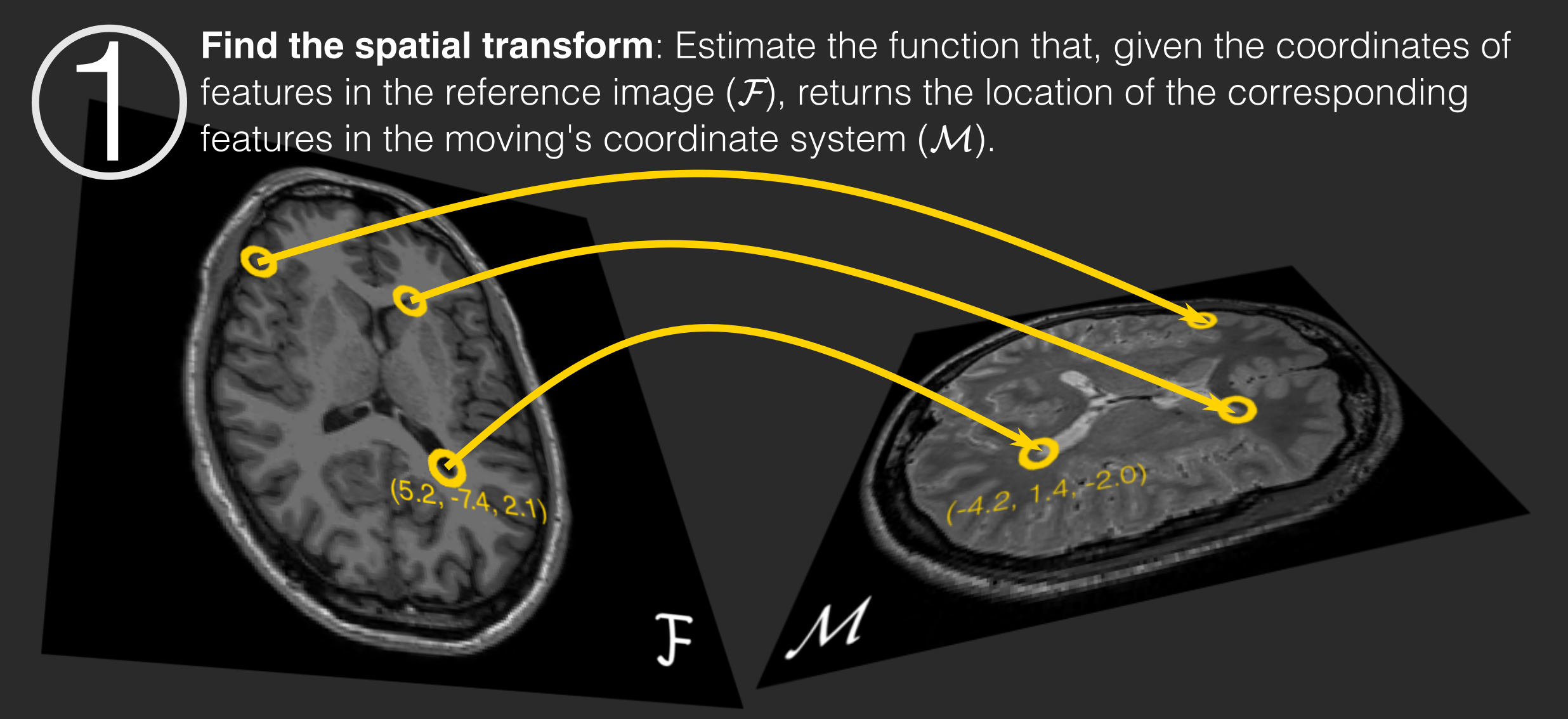
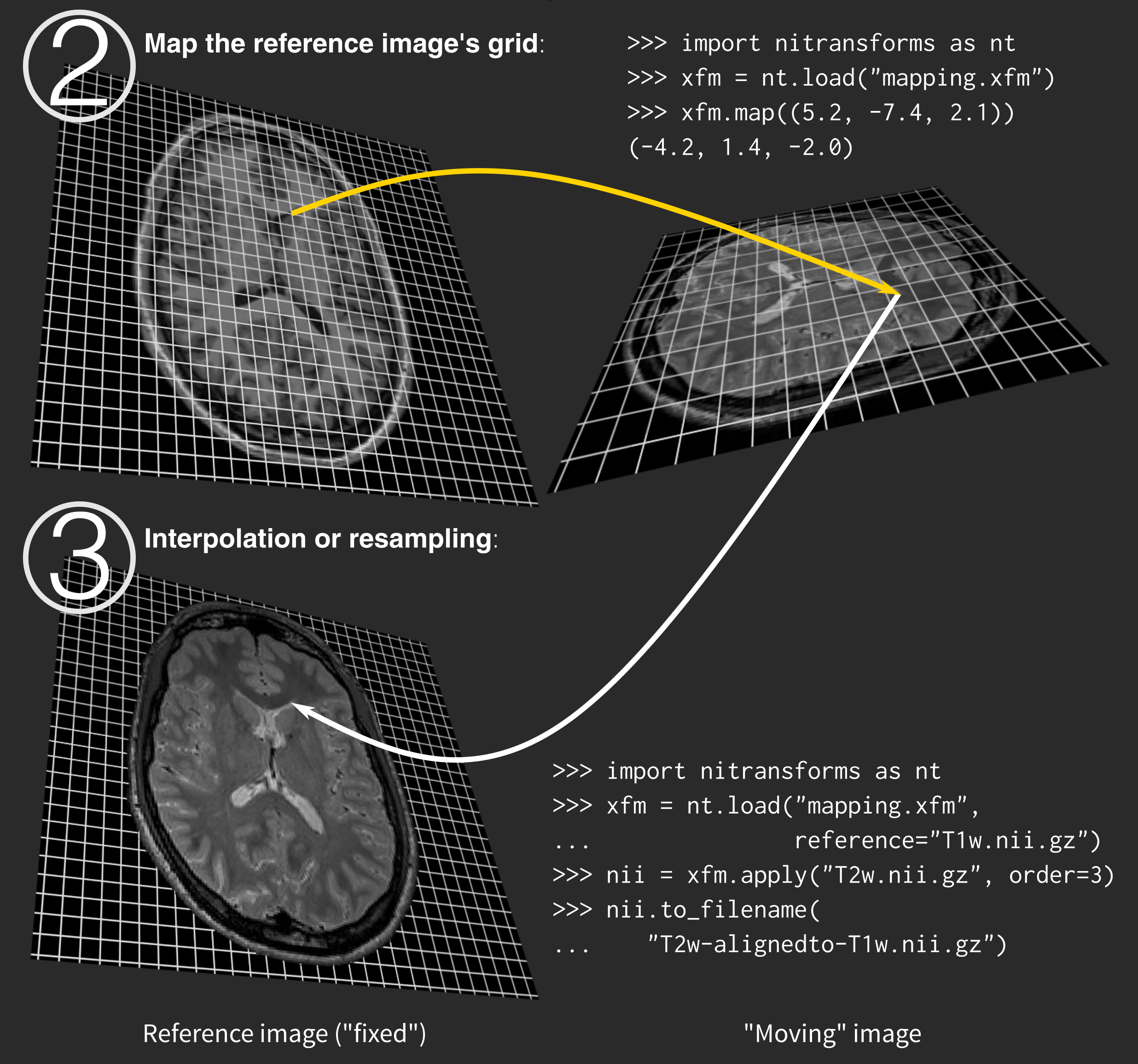
Spatial transforms
$T\colon \mathcal{F} \subset \mathbb{R}^n \to \mathcal{M} \subset \mathbb{R}^n$
$\vec{x} \mapsto \vec{x}' = f(\vec{x}).$